Neighborhood data is not a description of a place; it's a measurement made using a chosen boundary, a particular source, and an uncertainty level. Census tracts are statistical geographies, not necessarily neighborhoods recognized by residents, and estimates attached to them shouldn't be mistaken for exact counts or parcel-level facts (U.S. Census Bureau, ACS Researchers' Handbook).
Useful neighborhood analytics start by naming the geography, matching attributes to the decision, and testing whether the data can support the conclusion. That means keeping estimates and margins of error together, checking how results change across boundaries, and asking who or what is missing from the dataset before treating an apparent pattern as a market signal.
- Define the unit: A tract, block group, ZIP code, service radius, and custom polygon describe different areas.
- Choose attributes for the decision: Demographic, property, environmental, and behavioral indicators answer different questions.
- Validate before ranking: Sampling uncertainty, boundary effects, and uneven data coverage can distort comparisons.
- Keep the limits visible: An area-level pattern isn't automatically true of each household or parcel within it.
Neighborhood data becomes useful when its geography and uncertainty stay attached to the conclusion. That discipline matters whether you're comparing communities, screening properties, or planning a service area.
What Neighborhood Data Actually Means
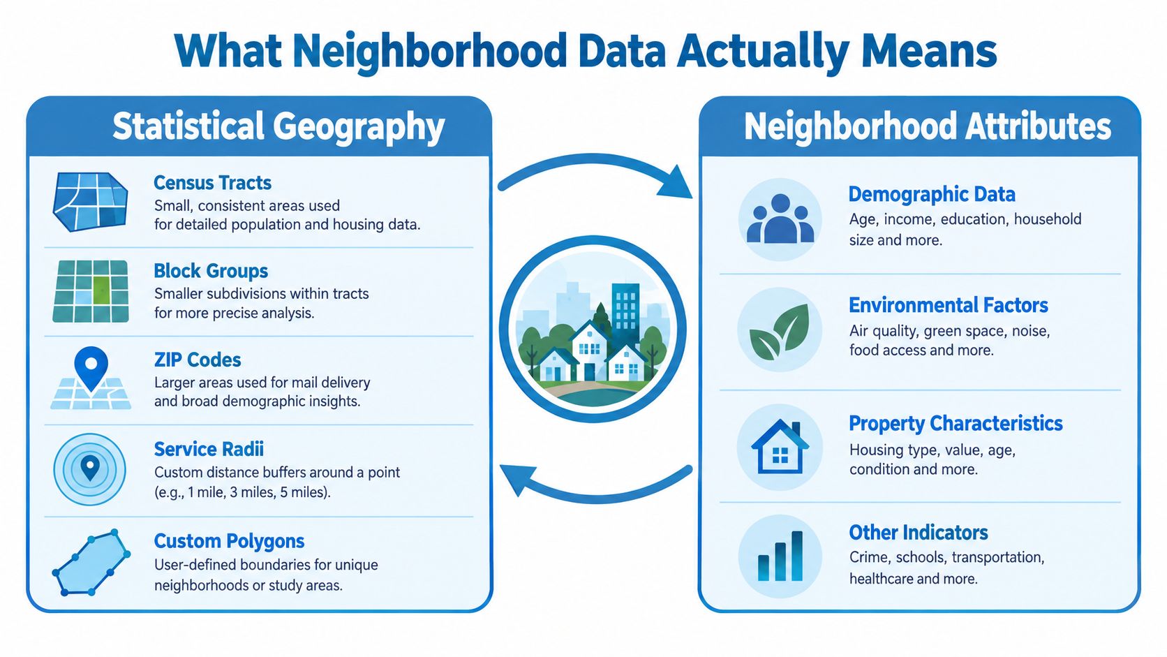
Neighborhood data combines a defined geography with attributes measured for that area or for properties within it. The geography might be a census tract, block group, ZIP code, service radius, or custom polygon. The attributes might describe residents, housing, hazards, ownership, access, or activity. Neither layer means much without the other: a statistic without a declared boundary is hard to interpret, while a boundary without relevant attributes can't answer an operational question.
A neighborhood isn't a single standardized statistical unit. The Census Bureau describes tracts as statistical geographies designed to make local conditions measurable and comparable, not as definitive boundaries for locally recognized neighborhoods (Census Bureau history of tracts). Block groups, ZIP codes, municipal boundaries, and real-estate market areas may overlap, diverge, or serve different purposes. Analysts should state which one they've used rather than letting the word “neighborhood” imply an agreed boundary.
Define the measurement before using it
Start by identifying the geographic unit and the level at which each attribute was measured. A tract-level estimate describes an area; it doesn't establish the characteristics of a specific household. A parcel record can describe a property, but it doesn't automatically explain the wider social or environmental conditions around it.
Then match the attribute to the decision. Demographic estimates may help characterize a market or service area. Property and ownership records can support parcel screening. Environmental layers can identify area-level exposure, but they can't by themselves tell you whether a particular household can recover from a hazard.
Practical rule: Record the geography and source alongside every neighborhood attribute. If the unit gets dropped during an integration, downstream users can mistake an area estimate for a property fact.
Readers exploring local character alongside statistical measures can find your ideal Puerto Rico community. The same principle applies in any location: a place's identity and a data provider's geographic unit may not draw the same boundary.
Neighborhood analysis therefore starts as a measurement problem, then becomes a product decision. The analyst's job is to make clear what the data can answer, what it cannot, and how much uncertainty travels with the result.
The History Behind Small Area Statistics
Small-area statistics were built to make local comparisons consistent, not to define every community's boundaries. Their history shows why analysts need to treat census geographies as measurement units rather than direct maps of neighborhood identity.
The first recorded small-area geographic units in U.S. Census Bureau history appeared around the 1890 census, when sanitary districts were organized within city wards for a special vital-statistics study. In 1906, Walter Laidlaw proposed permanent small geographic areas for consistent comparisons over time. Before the 1910 census, he divided New York City into 40-acre districts. In 1909, the Census Office adopted the tract concept and extended tract-based tabulation to seven other cities with populations above 500,000: Baltimore, Boston, Chicago, Cleveland, Philadelphia, Pittsburgh, and St. Louis (Census Bureau article on the centennial of census tracts).
The effort responded to a measurement problem: comparisons become difficult when geographic boundaries shift between data collections. After the 1930 census, the Bureau recognized the need for standardized boundaries and issued its first census-tract criteria in 1934. Tracts became an official geographic entity in the 1940 census, allowing population and housing statistics to be reported for smaller areas.
Wider coverage, more frequent estimates
Census-block tabulation, added in 1940, later supported block-group and block-level products for finer geographic analysis. Demand for nationwide small-area information increased from the 1970s, partly because legislative redistricting required broader coverage. By 2000, every U.S. county had been subdivided into census tracts, compared with an initial system covering about 25% of U.S. land area (Census Bureau working paper on small-area data).
In 2010, the American Community Survey (ACS) replaced the decennial census long form and began providing small-area estimates more often than once every ten years. Historical tract-level data is available from 1940 onward for metropolitan areas that were tracted. Comparable block-level data is available for the 1970, 1980, 1990, 2000, and 2010 decennial censuses (Census Bureau decennial census data products).
These changes expanded coverage and frequency, but they did not make census boundaries equivalent to community boundaries. Tracts can be revised as populations shift, so trend analysis may require boundary normalization or geographic crosswalks. A local guide can help readers find your Abbotsford neighborhood, while census geography remains a separate statistical framework. The distinction matters: neighborhood names support local orientation, but do not establish that two datasets measure the same place.
Core Attributes That Power Neighborhood Analysis
Neighborhood attributes are useful only when the measurement level and decision match. A demographic estimate may describe a population within a statistical area; an ownership record may describe a particular parcel. Treating those as equivalent creates false precision.
The ACS 5-year estimates provide indicators such as race and ethnicity, poverty, age, education, and language barriers at tract or block-group scale. Block groups are often used for environmental and demographic screening because they preserve more local detail than counties or cities. They typically contain about 600–3,000 residents, and the U.S. contains more than 200,000 block groups (EPA EJScreen report guide). Because the ACS 5-year product supports small geographic areas, its estimates can also carry substantial uncertainty; that limitation belongs with the attribute, not in a footnote after a score is deployed (EPA EJScreen fact sheet).
| Attribute Family | Typical Source | Geographic Unit | Primary Use Case |
|---|---|---|---|
| Demographic | ACS estimates, including population, age, education, poverty, and language indicators (demographic data overview) | Tract or block group | Market context, service planning, and screening |
| Housing and tenure | ACS housing estimates and property records | Tract, block group, or parcel | Housing mix, owner-occupancy context, and property targeting |
| Economic | ACS income indicators and property valuation records | Tract, block group, or parcel | Affordability context and underwriting inputs |
| Environmental | Hazard and environmental screening layers | Block group, tract, parcel, or custom area | Exposure screening and risk review |
| Mobility and access | Location, road, amenity, and activity data | Block group, service area, or custom polygon | Site selection and delivery coverage |
| Property and ownership | Property, ownership, mortgage, lien, and listing records | Parcel | Due diligence, portfolio review, and owner contact |
| Behavioral | Aggregated activity or service-use signals | Provider-defined geography | Demand patterns and operational planning |
Keep the unit attached to the attribute
Property and ownership data can bring analysis down to the parcel, while demographic or environmental estimates may remain tied to larger areas. That combination can be useful, but it doesn't convert an area statistic into a household-level observation. Analysts should retain the original geographic identifier and source for each attribute, even when they join it to a parcel.
A composite index also needs its components and interpretation. For example, EPA's EJScreen Demographic Index averages the share of residents with low incomes and the share of people of color, then reports relative standing in a national percentile context (EJScreen technical documentation). That score can help screen locations; it isn't an absolute measure of neighborhood quality or a substitute for investigating the underlying measures.
Quality, Uncertainty, and the Geography Problem
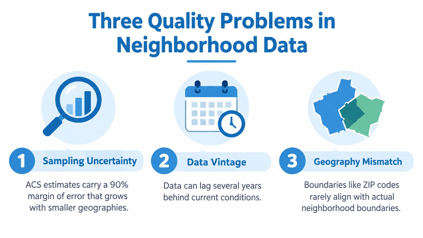
Three distinct problems determine whether neighborhood data can support a decision: sampling uncertainty, boundary sensitivity, and representativeness. A polished map doesn't resolve any of them.
Sampling uncertainty
ACS estimates are measurements with uncertainty, not exact counts. Published ACS estimates include a 90% margin of error (MOE), and the MOE generally becomes larger relative to an estimate when the underlying quantity is small. Rare events, small demographic groups, and low-count property segments are therefore especially unstable (ACS Researchers' Handbook).
Store the estimate and its MOE together, and calculate the confidence interval as estimate ± MOE. Don't rank two areas as meaningfully different when their intervals overlap in a way that makes the difference statistically indistinguishable. For modeling, an MOE can inform observation quality or help down-weight noisy labels. Aggregating adjacent areas may reduce uncertainty by increasing the effective sample size, but it also changes the geographic question being asked.
Boundary sensitivity
The modifiable areal unit problem (MAUP) means that correlations, rankings, accessibility measures, and apparent concentrations can shift when an analyst changes geographic scale or boundary configuration, even if the underlying observations stay the same. Scale effects come from aggregating into larger units; zoning effects come from changing the shapes or arrangement of the areas. Research on neighborhood proxies recommends testing alternative spatial structures rather than assuming one census geography represents every real neighborhood (research on neighborhood proxies and MAUP).
Compare results across parcel, block-group, tract, and service-radius resolutions where the decision warrants it. Track whether model effects, rankings, or hotspots persist. A tract-level score should not become a parcel-level claim.
Representativeness and vintage
A dataset can be technically complete and still describe activity unevenly. Curb-management research warns that data-collection tools may be deployed first in better-resourced neighborhoods, leaving inconsistent signage or incomplete records that make underserved communities appear to have less demand. Historical redlining can also compound current environmental exposure, so a contemporary risk layer may miss part of the context that shaped present conditions (equity considerations in curb management).
Audit coverage, missingness by geography and income or race proxy, update latency, and boundary changes. Ask whether “no record” means no activity or activity the system didn't observe. For an example of how a property-data provider explains its collection approach, review RentReboot's listing detection process. Spatial joins and layer choices should also be documented; GIS data layers can be part of that workflow, but they don't replace validation.
Integration Patterns for Neighborhood Data
Choose an integration pattern based on record volume, freshness needs, and whether the user is waiting for a result. An interactive property lookup and a portfolio-wide model refresh have different operating constraints; forcing both through one delivery path often adds avoidable complexity.
| Pattern | Best For | Typical Latency | Freshness Model |
|---|---|---|---|
| Low-latency API | Underwriting lookups, portal search, pre-qualification, and other interactive property or small-list queries | Designed for request-time responses; confirm service targets with the provider | Provider-managed updates, queried as needed |
| Bulk delivery | Portfolio monitoring, model training, and analytics warehousing | Background processing; not dependent on per-record response time | Scheduled files or data warehouse refreshes |
| Custom matching and enrichment | Records without a clean parcel identifier, or inputs requiring resolution to canonical property records | Depends on matching workflow and delivery method | Enrichment run on demand or as a batch |
Match the pattern to the workflow
Use an API when a person or application needs an attribute bundle while making a decision about a single property or a short list. That can support interactive underwriting or property search, provided the provider's measured latency meets the product requirement. Don't assume “API” guarantees a particular response time; test the actual endpoint under expected load.
Bulk delivery through S3, Snowflake, or flat files is better suited to jobs where the system processes many records without a user waiting for each result. Portfolio refreshes and model-development pipelines can use scheduled datasets, with full-record refreshes sometimes simpler to operate than reconciling changes record by record. The tradeoff is that batch workflows work on the latest delivered snapshot, not necessarily the latest record available from a live service.
Custom matching is appropriate when an analyst has an address, partial property description, or another identifier that doesn't cleanly map to a parcel ID. Resolve the input to a canonical property record before attaching neighborhood attributes, and preserve match confidence and source identifiers so a fuzzy join doesn't masquerade as certainty.
Decision rule: Choose by volume, freshness, and interaction pattern. If the workflow is per-record and user-facing, evaluate an API. If it's recurring and portfolio-scale, evaluate bulk delivery. If identifiers are messy, solve matching before debating the delivery format.
How Teams Use Neighborhood Data in Practice
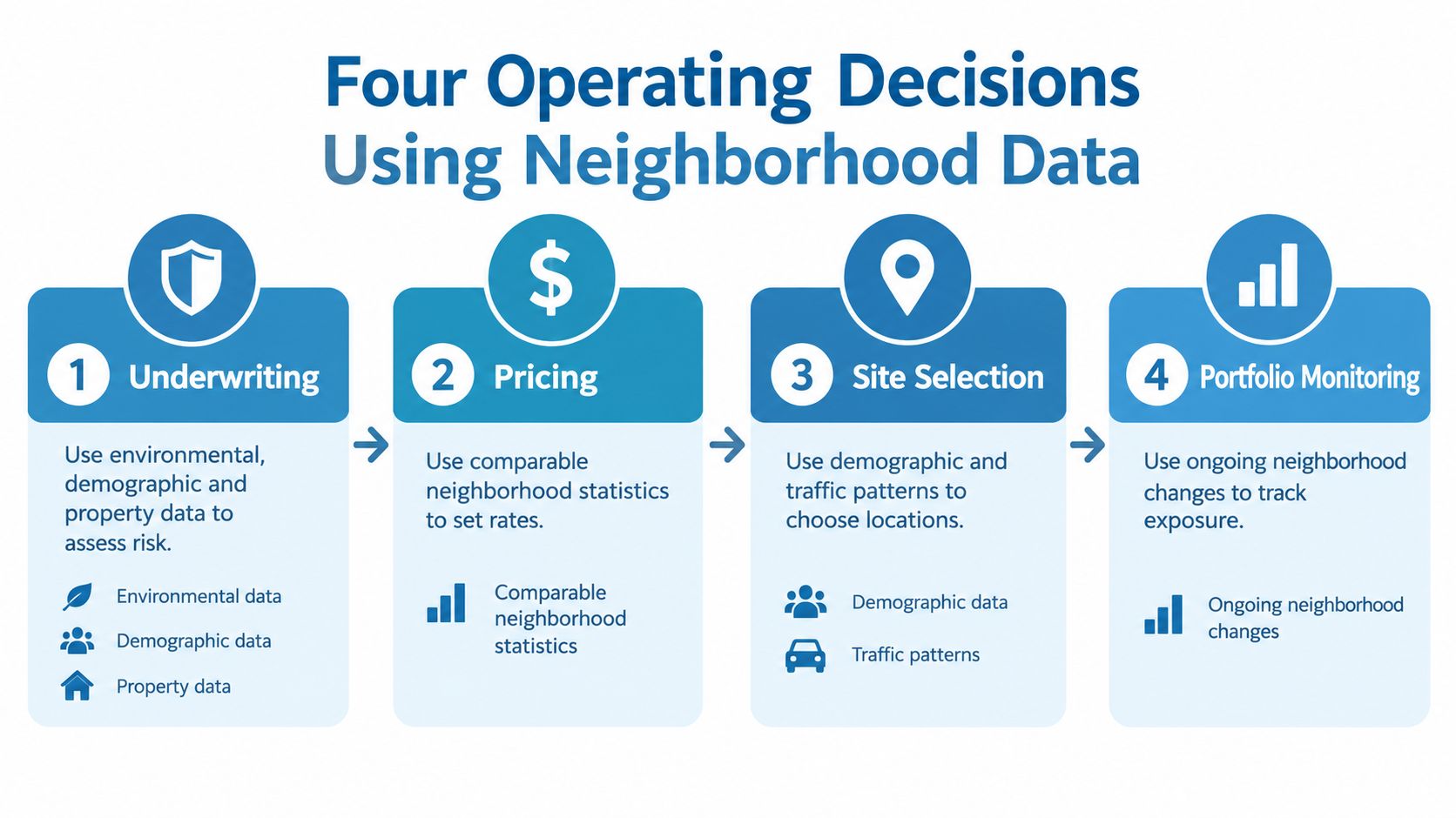
The operational value comes from connecting each signal to a specific decision, not from collecting the largest possible attribute bundle. Underwriting, marketing, risk modeling, and portfolio monitoring may use overlapping data, but they shouldn't treat the same field as equally reliable or relevant in every workflow.
Underwriting and marketing
Underwriting uses property characteristics alongside area-level demographic and environmental context to support risk tiers or loan-term review. A composite index can show a location's relative position, such as a national percentile, but it shouldn't be mistaken for an absolute risk measure. Analysts should inspect the component indicators and uncertainty before using an area score in a property decision.
Marketing and lead generation combine demographic and tenure context with property and owner records to prioritize outreach. Area-level propensity signals can help identify where a campaign may fit, while verified contact information and property-level evidence are needed to reach a specific owner. The distinction matters: an area profile can help prioritize, but it doesn't prove an individual's intent. Teams considering acquisition targeting can explore how demographics drive property acquisition decisions.
Risk modeling and portfolio monitoring
Risk modeling should separate hazard exposure from vulnerability and capacity to recover. Join hazard information to parcel-level structure and ownership records where available, then preserve the provenance and geographic unit of every input. A single score can obscure whether risk comes from physical exposure, building conditions, or constraints on recovery.
Portfolio monitoring uses recurring updates to identify accounts whose property or neighborhood context may have changed. Pre-foreclosure, equity, ownership, and hazard indicators can support review queues, but an alert is a reason to investigate, not proof that a borrower or property has changed status.
A sample query could select owner-occupied single-family parcels in a target county where the tract's environmental index exceeds the 80th national percentile and assessed equity is above a chosen threshold. The result can be routed to a contact-enrichment workflow, with the tract-level index kept distinct from parcel-level ownership and equity fields.
The workflow becomes clearer when each stage is treated as a separate decision: assess an application, set pricing, select a site, or monitor a portfolio. A short video can add context on how such analytics workflows are organized:
Inside the Neighborhood Risk Question
A neighborhood average can hide which residents and properties face the greatest exposure. In a study of 276 cities across eight Latin American countries, 80% showed educational-attainment disparities in flood exposure; 24.0% of neighborhoods with the lowest educational attainment were in flooded areas, compared with 5.6% of neighborhoods with the highest educational attainment (study of flood-exposure disparities across Latin American cities).
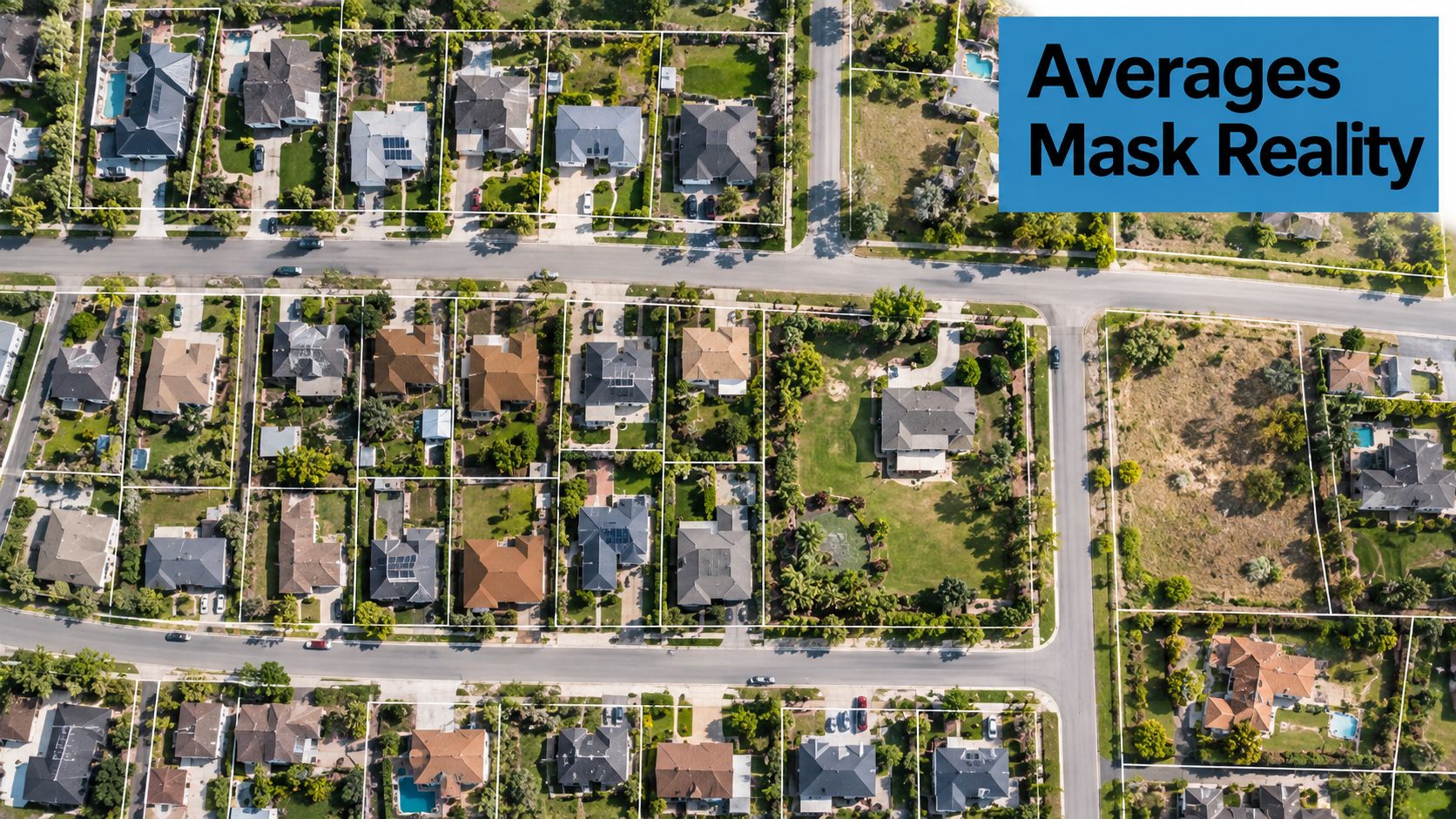
The figures illustrate why a neighborhood label isn't an adequate risk decision. An area average can conceal differences between properties, households, and their ability to respond. Exposure describes contact with a hazard; resilience depends on factors that a hazard score alone may not measure.
Move from area screening to property context
For lenders, insurers, investors, and logistics operators, the useful question isn't just whether a neighborhood is safe or unsafe. It's which properties are exposed, which owners can be reached, and which interventions could reduce risk.
A stronger workflow overlays frequently refreshed property and ownership records with hazard, infrastructure, and social-vulnerability layers. It then separates current exposure from adaptive capacity, and flags where local review is needed rather than treating an area score as a definitive verdict. Depending on the use case, that review may consider building condition, tenure, insurance capacity, tree cover, access to cooling, or pressure from mortgages and liens.
This approach also changes how teams interpret missing data. No record can mean no observed activity, not no activity. A model that assigns low risk or low demand to an unobserved property may systematically exclude the places where its inputs are weakest.
A useful neighborhood score should direct attention to properties and people who need closer examination. It shouldn't turn a complex exposure pattern into a label that closes the case.
Measurement Discipline and Ethical Guardrails
Defensible neighborhood analytics keep geography, uncertainty, and data coverage visible from ingestion through decision. A dashboard can't make a weak measure reliable by giving it a clean color scale.
Use this operating checklist:
- Label the unit: Store the tract, block group, parcel, ZIP code, or custom geography with each record.
- Keep uncertainty attached: Preserve each estimate with its margin of error when one is available.
- Audit coverage: Compare missingness across geography and income or race proxies before trusting rankings.
- Interpret absence carefully: Decide whether no record represents no activity or activity the source didn't observe.
- Document provenance: Make the source and components of any score transparent when it influences lending or insurance decisions.
- Minimize personal data: Use only the consumer information required for the intended recommendation, and monitor outcomes for disparate impact across protected classes.
These controls make comparisons more defensible and give reviewers a way to trace how an output was produced. They also help teams catch cases where boundary changes, stale updates, or uneven observation have altered a result without changing its headline score.
Neighborhood data is powerful precisely because it's approximate. Teams that keep the uncertainty visible can use it to guide investigation and decisions without pretending that an area-level measure tells the whole story.
BatchData provides property and ownership records, valuations, contact enrichment, and neighborhood-related attributes through API and bulk-delivery options. If your team is building neighborhood analytics, visit BatchData to assess whether its property data and matching workflows fit your integration and decision needs.