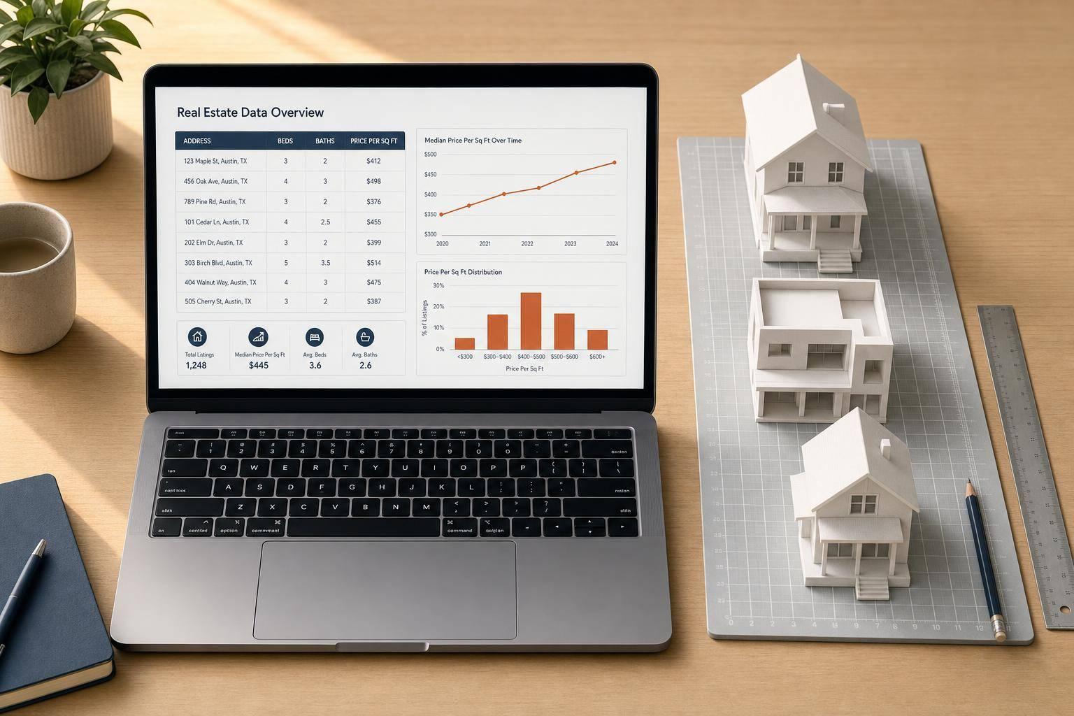
Real estate data is rarely ready for analysis the moment it leaves a CRM, lead source, MLS export, or internal pipeline. Square footage is missing. Prices contain obvious keying errors. Fields are structured just well enough to look usable - until your team tries to model pricing, route leads, or compare neighborhoods at scale.
That is what makes this walkthrough valuable: it does not treat analysis as a visualization exercise. It starts where real property operations usually start - with messy listing data - and shows how to turn it into something dependable enough for decision-making.
The video uses a synthetic housing dataset in pandas, then walks through a complete workflow: generating records, introducing realistic problems, cleaning the data, creating better metrics, and summarizing the market by neighborhood. For technical teams, the bigger lesson is not just pandas syntax. It is the discipline of building an analysis pipeline that can survive imperfect inputs.
Why This Matters for Real Estate Teams
If you work in acquisitions, lead scoring, home services targeting, valuation, or proptech product development, bad data does more than create ugly spreadsheets. It creates operational drag:
- Investors chase false pricing signals
- Sales and marketing teams target the wrong owners
- Analysts build reports off distorted averages
- Developers spend time patching one-off data issues instead of shipping systems
The tutorial’s structure mirrors a useful real-world pattern:
- Build or ingest a dataset
- Profile it before trusting it
- Fix missing values with business context
- Contain outliers without destroying row-level history
- Normalize raw values into comparable metrics
- Summarize patterns by segment
- Visualize results for fast interpretation
That sequence is far more important than any single function.
Key Takeaways
- Profile before you analyze. Check shape, missing values, and descriptive statistics before building charts or models.
- Impute with context, not convenience. Filling missing square footage by neighborhood median is more defensible than using one global average.
- Outliers can ruin pricing analysis. A few inflated prices can distort means, correlations, and segment thresholds.
- Capping is often better than deleting. When a row is still useful but one field is wrong, clipping extreme values preserves dataset size and structure.
- Price per square foot is more useful than raw price alone when comparing unlike properties.
- Correlation helps prioritize features, not prove causation. Strong relationships can guide investigation, but they do not explain market behavior by themselves.
- Quantile-based price tiers are useful for balanced segmentation when you want evenly sized groups for reporting.
- Neighborhood summaries turn row-level noise into market intelligence your ops or acquisitions team can act on.
- Simple visuals still matter. A scatter plot and a bar chart can validate assumptions faster than a dense spreadsheet.
- Action item: If you manage listing or ownership datasets, turn this into a repeatable notebook or pipeline so data cleaning happens the same way every time.
The Real Lesson: Synthetic Data as a Safe Stand-In for Production Problems
The video begins by generating 250 synthetic home listings with fields such as neighborhood, bedrooms, bathrooms, square footage, year built, days on market, and listing price. That might sound basic, but it is a smart teaching setup.
Synthetic data creates a controlled environment where you can:
- test cleaning logic safely
- reproduce results with a fixed random seed
- introduce known errors on purpose
- verify whether your detection methods actually catch those errors
For data teams, this is more than beginner-friendly. It is a useful engineering habit. Before you deploy logic into a production property workflow, it helps to validate your assumptions against a dataset where you already know which records are broken.
The video also emphasizes reproducibility by seeding the random generator. That matters because repeatable outputs make debugging, collaboration, and QA much easier - especially when multiple stakeholders are reviewing the same notebook.
Start with Data Profiling, Not Assumptions
A common mistake in real estate analytics is jumping from file import to dashboard. The tutorial avoids that by taking a first pass through the dataset with three basic checks:
- row and column count
- missing-value counts
- summary statistics on price
This is simple, but strategically important.
Why shape matters
Knowing the dataset has 250 rows and 8 columns is not just bookkeeping. It confirms the import worked as expected and gives context for later decisions. A missing-value issue across 15 rows means something very different in a 250-row file than it would in a 250,000-row export.
Why missing-value counts matter
The square footage column contains 15 missing values. That is enough to affect downstream metrics like:
- price per square foot
- average home size by neighborhood
- correlation between size and price
- model features for valuation
Without this check, a team could unknowingly build comparisons on incomplete data.
Why descriptive statistics matter
The price summary reveals a maximum value far above the upper quartile. That is the first signal that some prices may be invalid. In property datasets, this happens constantly:
- extra zeros added during manual entry
- mismatched decimal handling
- duplicate record merges
- stale or malformed source values
The broader lesson is clear: descriptive stats are not a formality - they are an early-warning system.
Imputing Missing Square Footage the Right Way
One of the strongest parts of the tutorial is the decision to fill missing square footage using the median within each neighborhood, rather than one average across the full dataset.
That is a better method because housing stock is local.
A missing size value in a dense neighborhood with smaller homes should not be filled using the same benchmark as a neighborhood with larger detached properties. Group-level imputation respects the structure of the market.
Why median beats mean here
The video uses the neighborhood median, not the mean. That choice matters because medians are less sensitive to unusually large or small homes. If your goal is to create a stable replacement value, the median is often the safer default.
Why groupby plus transform is so useful
The pandas pattern highlighted in the tutorial is effective because it calculates a neighborhood-level statistic while keeping alignment at the row level. In operational terms, that means you can fill missing values without collapsing the dataset into a summary table.
For real estate data pipelines, this is exactly what you want: preserve every record while enriching it with local context.
Where teams should be careful
This method is strong, but it still has limits:
- If a neighborhood has very few records, its median may be unstable
- If neighborhoods are mislabeled or inconsistently named, the imputation can become unreliable
- If square footage is missing systematically - say, only for certain property types - you may need a more advanced strategy
Those caveats are not addressed in depth in the video, but they are worth keeping in mind for production use.
Handling Price Outliers Without Throwing Away Records
The tutorial uses the interquartile range (IQR) method to identify high-price outliers. It then caps extreme prices at the calculated upper bound instead of deleting those rows.
This is a practical decision for real estate operations.
Why outlier detection matters so much in housing data
A handful of bad prices can distort:
- average listing price
- neighborhood rankings
- price tier assignments
- model coefficients
- forecast assumptions
- sales team expectations
If one entry is inflated by a factor of ten, it does not just look wrong - it actively contaminates your analysis.
Why IQR is a solid default
The IQR method is robust because it focuses on the middle range of the data rather than assuming a normal distribution. That makes it especially useful in real estate, where prices are often skewed.
The tutorial identifies five outliers, which matches the number intentionally injected into the dataset. That confirmation is important: it shows the method worked on the known problem.
Why capping can be better than dropping
Deleting outliers is tempting, but it can introduce new problems:
- smaller datasets
- broken joins with other tables
- lost metadata from otherwise valid records
- reporting inconsistencies across teams
Capping preserves the row while limiting the damage from the bad value.
That is often the right move when the record itself is real, but the price field is not.
The tradeoff
Capping is not perfect. It reduces skew, but it also compresses true variation at the top end. In luxury markets, some high prices are legitimate. A production pipeline should ideally distinguish between:
- obvious data-entry errors
- valid premium listings
- special-use properties
The video does not go into that nuance, which is understandable for a foundational tutorial. Still, teams applying this approach in higher-end markets should review flagged records rather than auto-cap everything without context.
Why Price Per Square Foot Is a Better Comparison Metric
Raw price is easy to read but hard to compare. A 900-square-foot condo and a 3,200-square-foot suburban home do not belong in the same pricing conversation unless you normalize for size.
That is why the tutorial creates price per square foot after cleaning the data.
This is one of the most useful metrics in real estate analysis because it helps answer questions like:
- Which neighborhoods command a premium relative to home size?
- Which listings may be overpriced for their footprint?
- Where does marketing or acquisition strategy have room to adjust?
- Which segments appear undervalued compared to nearby comps?
Why cleaning comes first
This is also a good example of sequencing. The tutorial calculates price per square foot only after:
- filling missing square footage
- capping implausible prices
That order matters. If you create derived metrics before fixing core fields, you simply spread the errors into a new column.
For data teams, the principle is simple: clean source variables before creating business metrics from them.
Correlation Analysis: Useful, but Easy to Misread
The video then runs a correlation analysis across numeric variables and sorts them by relationship to listing price. Square footage emerges as the strongest driver, with bedrooms and bathrooms also positively related. Days on market and year built show weaker relationships.
That result makes intuitive sense. Larger homes generally cost more.
But this section deserves a little extra interpretation.
What correlation is good for
Correlation is useful for:
- quick feature screening
- identifying likely drivers
- spotting redundancy across variables
- guiding exploratory analysis
If square footage has the strongest relationship with listing price, that tells you where to focus first.
What correlation does not tell you
Correlation does not prove:
- that one variable causes another
- that the relationship is linear in all segments
- that the effect holds equally across neighborhoods
- that omitted variables are unimportant
For example, square footage may dominate in a synthetic dataset, but real markets are shaped by many factors not specified in the video, such as lot size, school districts, renovation quality, zoning constraints, and property type.
So while the correlation matrix is useful, it should be treated as a directional tool - not a final pricing model.
Balanced Price Tiers Can Improve Reporting
Next, the tutorial creates four price tiers using quantile-based binning. Instead of fixed dollar ranges, it splits listings into roughly equal-sized groups such as budget, mid-range, upper-mid, and premium.
This is a smart reporting move.
Why quantile tiers are useful
Fixed pricing bands can produce lopsided buckets. If your market is clustered tightly in one range, one tier may hold most of the records while another barely gets used.
Quantile-based tiers solve that by balancing group counts.
That makes them especially useful for:
- operational dashboards
- lead-routing rules
- sales coverage planning
- market segmentation summaries
- comparing behavior across equally represented pricing bands
Where fixed bands may still be better
In some business contexts, quartiles are less intuitive than explicit price ranges. Sales leaders may care more about strategic cutoffs like:
- under $250K
- $250K–$500K
- $500K–$1M
- over $1M
The right method depends on the use case. Quartiles are excellent for statistical balance. Fixed bands are often better for business communication.
The tutorial’s choice fits analysis well, especially for an evenly segmented first pass.
Neighborhood Summaries Turn Raw Data into Strategy
One of the most practical sections in the video is the grouped summary by neighborhood. Instead of stopping at record-level analysis, it aggregates into metrics that decision-makers can actually use:
- listing count
- average cleaned price
- average price per square foot
- average days on market
This is the point where a notebook starts to become operationally relevant.
Why this summary works
It combines three kinds of intelligence:
- Market scale through listing count
- Value level through average price
- Normalized pricing through average price per square foot
- Velocity through days on market
That mix gives a more complete view than price alone.
A neighborhood with high average price may still be less attractive if homes sit longer, while a neighborhood with moderate average price but strong price-per-square-foot trends may indicate tighter demand or different housing stock.
What operators can do with this
Depending on the team, a summary like this can support:
- acquisition targeting
- outbound marketing prioritization
- valuation sanity checks
- market-entry analysis
- sales territory planning
For example, a home services company might focus first on neighborhoods with strong volume and stable pricing, while an investor may look for areas with lower averages but favorable turnover signals.
Visuals Still Matter - Even for Technical Teams
The tutorial ends with two charts:
- a scatter plot of square footage versus listing price
- a bar chart of average price by neighborhood
These are standard visuals, but they do real work.
What the scatter plot confirms
The scatter plot helps validate the basic relationship between size and price. After cleaning, the upward trend is easier to see because the extreme errors no longer dominate the chart.
This is an underrated benefit of cleaning: visualizations become interpretable.
What the bar chart adds
The neighborhood bar chart compresses a lot of data into a form executives and operators can scan quickly. It is not a substitute for deeper analysis, but it is useful for fast comparison.
Together, the two visuals serve different audiences:
- the scatter plot supports exploratory analysis
- the bar chart supports summary communication
That combination is a good pattern for internal reporting.
What the Tutorial Does Well
This walkthrough stands out for a few reasons.
It teaches workflow, not just syntax
The biggest value is the sequencing. The video does not throw isolated pandas commands at the viewer. It demonstrates a realistic order of operations.
It uses deliberately messy data
That is closer to how real property records behave. Clean toy examples are easy to follow but often fail when applied to exports from live systems.
It introduces robust defaults
Neighborhood median imputation, IQR-based outlier detection, clipping, and normalized pricing are all sensible baseline methods.
It stays practical
The output is not abstract. It ends with summaries and visuals that a real team could present or build on.
What’s Not Specified in the Video
For teams looking to productionize this workflow, a few areas are not specified in the video:
- automated validation rules for incoming files
- handling duplicate listings
- standardizing neighborhood names
- merging listings with ownership, parcel, or contact data
- testing for low-confidence imputations
- managing legitimate luxury outliers
- packaging the notebook into a scheduled pipeline or API service
Those gaps do not weaken the tutorial. They simply mark the boundary between an introductory analysis workflow and a production data system.
How to Apply This Framework to Real Property Data
If you want to use the tutorial’s approach on live real estate data, adapt it into a repeatable framework:
1. Audit every new dataset
Check structure, null rates, datatypes, and descriptive stats before using it downstream.
2. Impute with local logic
Use neighborhood, ZIP code, property type, or bed/bath segments instead of one-size-fits-all fills.
3. Flag and review price anomalies
Start with IQR or percentile rules, then refine based on asset class and market.
4. Create normalized metrics early
Price per square foot, days on market bands, and local ranking metrics help reduce misleading comparisons.
5. Aggregate for action
Neighborhood, ZIP, or county summaries are easier for ops, acquisitions, and leadership to use than row-level tables.
6. Separate analysis rules from business rules
A statistically convenient threshold is not always the right one for sales or underwriting decisions.
Conclusion
The core value of this tutorial is not that it teaches pandas on a housing dataset. It is that it models a clean analytical mindset for real estate data work.
The process is straightforward but powerful:
- inspect the data before trusting it
- repair missing fields using local context
- contain bad outliers without losing records
- create normalized metrics for fair comparison
- summarize results at the market level
- use visuals to validate and communicate findings
For real estate investors, operators, and developers, that workflow is highly transferable. Whether you are analyzing listings, off-market opportunities, homeowner leads, or valuation inputs, the same rule applies: good decisions depend on clean, structured, and context-aware data.
And in property data, that cleaning step is not a side task. It is the foundation of everything that follows.
Source: "Real Estate Data Analysis with Pandas: Clean, Explore, Visualise" - Mathew K Analytics, YouTube, Aug 21, 2026 - https://www.youtube.com/watch?v=0f2jB5hcMT4