Query Optimization for Large Property Datasets

A property search portal can feel broken even when the application code is clean. A user selects a ZIP code, property type, value range, ownership filters, and mortgage details, then waits while the database evaluates a plan that looked cheap only on paper.

Query optimization for large property datasets requires more than adding an index. The database must estimate cardinality accurately, choose a workable join order, and return results through an API that doesn't repeatedly rescan the same records. At the scale of 155 million property records, SQL planning and API delivery are one latency problem.

• SQL decides what the database touches.
• Statistics determine whether the chosen plan is credible.
• Indexes and partitions reduce avoidable work.
• Cursor pagination prevents deep-page rescans.
• Workload history exposes plans that degrade after data changes.

How Cost-Based Query Optimization Actually Works

A lagging property portal usually has one of three problems: the query touches too many rows, the optimizer misjudges the rows it will touch, or the API asks the database to repeat expensive work. The first problem is visible. The second often hides inside an execution plan.

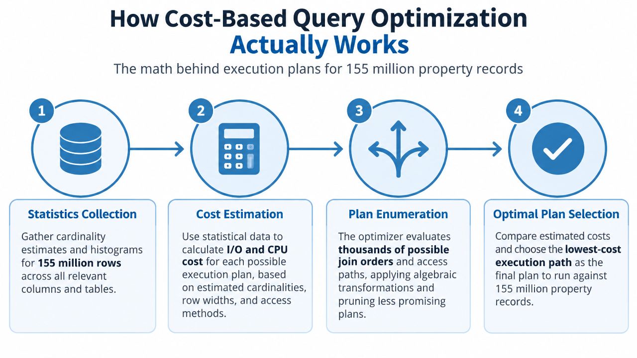
What selectivity tells the optimizer

Selectivity is the fraction of rows that satisfy a predicate. It ranges from 0.0 to 1.0, where 0.0 means no rows qualify and 1.0 means every row qualifies, as defined in Georgia Tech's cost-based query optimization material.

For a property search, a ZIP filter may be highly selective, while a broad property-type predicate may leave a large portion of the table. The optimizer uses those estimates to predict the cardinality of each intermediate result and compare candidate operators.

That choice often comes down to an index scan versus a sequential table scan. Oracle documents that index-scan cost includes B-tree levels, index leaf blocks scanned, and rows fetched through rowids, so the model accounts for both tree traversal and table access work. A selective predicate can favor an index. A broad predicate can make a sequential scan cheaper because fetching many scattered rows through an index creates extra work.

Microsoft SQL Server describes statistics as distribution information for table or indexed-view columns. The optimizer uses that information to estimate result-set cardinality and may choose an index seek instead of an index scan when it expects fewer rows to be touched, as explained in SQL Server statistics documentation.

Why estimates fail on property filters

The traditional approach relied heavily on base-table statistics and often assumed attribute independence. The 2002 ACM SIGMOD paper on exploiting statistics on query expressions challenged that model, showing why richer statistics matter when estimates move through filters and joins. The paper's central lesson remains practical: optimization quality depends on the cost model and on the granularity and freshness of the statistics feeding it. Read the original discussion in the ACM SIGMOD paper on statistics for query expressions.

Real estate filters frequently violate independence assumptions. Property type, geography, assessed value, sale history, and lien status can be correlated. If the optimizer estimates each predicate separately and multiplies assumptions that don't match the data, the error can grow across a multi-table plan.

A useful review resource for engineers preparing to diagnose these mechanics is top SQL questions from ThirstySprout. Treat interview-style explanations as a vocabulary check, then verify production behavior with actual plans and runtime measurements.

Reading EXPLAIN Plans for Property Search Queries

An EXPLAIN plan tells you what the optimizer expects to happen. An execution-analysis plan tells you what happened. You need both before changing SQL or indexes.

Start with the access path

Run the plan against the exact property-search shape, not a simplified query that removes the problematic filters. In PostgreSQL, use EXPLAIN (ANALYZE, BUFFERS) when production-safe execution is acceptable. In Snowflake, inspect the query profile and operator statistics rather than relying on a textual plan alone.

Look for these mismatches:

• Estimated rows versus actual rows: A large difference indicates a cardinality problem, stale statistics, or a predicate the model can't represent well.
• Sequential scans: A sequential scan may be correct for a broad filter, but it's suspicious when a highly selective, indexed predicate should narrow the result early.
• Rows removed by filter: Large removal counts show that the engine read data before applying a restriction that might have been pushed down.
• Join inputs: Check whether a large relation reaches a join before selective geography, property, or ownership predicates have reduced it.
• Buffers and spills: High buffer activity or disk spills can reveal memory pressure and data movement that the estimated cost hides.

Distinguish an index win from an index illusion

An index node doesn't automatically mean the query is efficient. The database may traverse the index, read many leaf blocks, fetch a large number of table rows, and perform additional filtering afterward. Oracle's explanation of index cost is useful here because it separates B-tree traversal, leaf-block work, and row retrieval instead of treating an index as a free shortcut.

Compare estimated and actual work at each node. If the plan expects a small row set but returns a much larger one, the optimizer may choose nested loops where a hash-oriented strategy would be safer. If the estimate is accurate but the index still causes extensive random access, a sequential scan may be the better design.

The PostgresGUI guide to analyze Postgres queries is a practical companion for reading EXPLAIN ANALYZE output and connecting plan nodes to observed execution behavior.

Use the following diagnostic sequence:

1. Confirm the starting relation. Identify which table or partition the engine reads first.
2. Trace predicate application. Find where ZIP, state, property type, value, and date restrictions take effect.
3. Follow row counts. Track the result size after every filter and join.
4. Inspect the expensive node. Separate CPU, I/O, sorting, hashing, and network exchange costs.
5. Test one change. Update statistics, rewrite a predicate, or alter one index, then compare plans and runtime.

The video below provides a visual introduction to execution-plan reasoning before you apply the same discipline to a live property query.

Indexing and Partitioning 155M Real Estate Records

Indexing a large property table works when the index matches the access pattern, while partitioning works when the query can eliminate entire data regions before evaluating row-level predicates. They solve different problems.

A composite index should reflect the filters users apply together, not an abstract list of popular columns. For a relational property table, a search pattern might look like this:

CREATE INDEX property_search_geo_type_value_idx
ON properties (zip_code, property_type, estimated_value);

Column order matters. Put the most reliable leading restriction first when it narrows the search and appears consistently in the workload. Don't create a wide composite index for every possible combination. Each additional index adds write, storage, and maintenance work.

For date-oriented access, use a separate structure when the workload frequently filters by recording or update date:

CREATE INDEX property_updated_idx
ON properties (updated_at);

Partitioning changes the unit of elimination. A table partitioned by state or county can allow the engine to skip unrelated geographic segments. In an S3-backed lake, the same principle applies through directory or file partitioning, for example by state and county, provided the query exposes those columns as usable predicates.

CREATE TABLE properties_partitioned
PARTITION BY LIST (state_code);

CREATE TABLE properties_ca
PARTITION OF properties_partitioned
FOR VALUES IN ('CA');

CREATE TABLE properties_tx
PARTITION OF properties_partitioned
FOR VALUES IN ('TX');

The syntax varies across PostgreSQL, Snowflake, and lakehouse systems, but the operating principle is stable: partition keys should match common pruning predicates. Partitioning by a column that queries rarely constrain creates management overhead without reducing scanned data.

Index Strategy	Best Use Case	Latency Impact
Composite B-tree index	Repeated equality and range filters such as geography, type, and value	Reduces row-level work when leading columns are selective
Single-column index	A frequently used, independently selective predicate	Helps targeted lookups, but may be weaker for combined filters
Geographic partitioning	Searches commonly constrained by state or county	Removes unrelated partitions before detailed filtering
Date partitioning	Incremental loads, recent updates, or historical slices	Limits scans to relevant time ranges

Statistics maintenance is part of indexing, not an afterthought. SQL Server describes statistics as distribution data used for cardinality estimation, so stale distributions can push the optimizer toward a poor access path even when the index itself is well designed.

Practical rule: Measure the query shape before adding an index. An index that helps a narrow property lookup can hurt a broad export by forcing expensive row retrieval.

For a broader explanation of tuning database performance the right way, focus on the same discipline: measure the workload, change one variable, and validate the resulting plan. Teams working with property APIs should also account for the data-access layer, as described in the complete guide to property data APIs.

Tuning Joins and Predicates for Complex Filters

Join order is often the largest source of opportunity and error in a property data query. A search that combines characteristics, ownership history, mortgage liens, and transaction records can produce very different intermediate result sizes depending on which relation the engine processes first.

Dynamic programming is one established approach. The optimizer compares join orders and retains a cheaper access path for each table or subexpression, as described in this material on database query planning and joins. A merge join becomes attractive when both inputs are already sorted on the join key, or when the inputs are small and cheap to sort.

Compare join alternatives

Join choice	Useful condition	Main risk
Nested loop	One side is small and the inner access path is cheap	Repeats work when the outer estimate is wrong
Hash join	Inputs are unsorted and the engine can build an in-memory hash structure	Memory pressure or spilling on larger inputs
Merge join	Inputs are sorted on the join key or sorting is inexpensive	Sorting cost can dominate when inputs are large

Write predicates so the optimizer can apply them as early as possible. Avoid wrapping indexed columns in functions when an equivalent range predicate exists. Keep join keys type-compatible, because implicit conversions can prevent efficient access and distort cost assumptions.

Subqueries also deserve scrutiny. A correlated subquery may execute in a way that repeatedly probes a large relation, while a carefully structured join or pre-aggregated relation can expose a clearer plan. Don't rewrite mechanically. Compare actual plans, because a modern optimizer may already transform some subqueries effectively.

Isolate the predicate that causes the regression

When a complex query becomes slow, remove one filter or join at a time and compare the plan. The goal isn't to create a permanently simplified query. It's to identify the condition that changes the chosen join order or access method.

A discriminative query pair keeps everything constant except one predicate. For example, hold the geographic and ownership filters steady, then compare a value range with a lien-status condition. If the second predicate causes estimated rows to collapse while actual rows remain high, you've found a likely estimation fault.

A recent benchmark study uses optimization potential to compare runtimes from optimal plans with plans selected by PostgreSQL, while a VLDB evaluation reports that order-of-magnitude gaps or worse occur routinely across systems for larger expressions. These findings support testing join-heavy workloads against optimal or near-optimal baselines rather than trusting a single successful benchmark, as documented in the AIDB benchmark paper.

Traditional benchmark queries may not stress join-order search enough. Use representative property workloads, vary predicates deliberately, and preserve the slow query's real data distributions.

API Pagination and Batching for High-Volume Delivery

A fast SQL query can still produce a poor product if the API requests deep offsets, returns oversized payloads, or holds a connection while serializing a massive result. Pagination is part of query optimization because the API's page contract determines how much database work each request triggers.

Replace offsets with stable cursors

Offset pagination is simple:

SELECT property_id, address, estimated_value
FROM properties
WHERE state_code = 'TX'
ORDER BY property_id
LIMIT 100
OFFSET 10000;

The problem is that the database may need to walk past earlier rows before returning the requested page. Deep offsets also become unstable when records are inserted or removed between requests.

Keyset pagination uses the last observed sort key:

SELECT property_id, address, estimated_value
FROM properties
WHERE state_code = 'TX'
  AND property_id > :last_property_id
ORDER BY property_id
LIMIT 100;

The cursor must match the ordering and index. If property_id isn't unique, use a tie-breaker such as a second stable column and encode both values in the cursor. Treat cursors as opaque API tokens, validate their filter context, and reject a cursor created for one search when the client changes the search criteria.

Choose delivery mode by workload

Consumer search needs small, predictable pages. Back-office exports need resumability, larger batches, and a delivery channel that doesn't force the API request to remain open.

• Interactive API pages: Return a bounded page, a cursor, and a has_more indicator.
• Bulk extraction: Create an asynchronous job and write partitions to S3, Snowflake, or flat files.
• Concurrent retrieval: Parallelize only across independent, bounded batches, with a queue that respects database and API capacity.
• Static attributes: Cache rarely changing property characteristics and invalidate them when the source update process changes.
• Volatile fields: Query ownership, listing, lien, or valuation fields through a freshness-aware path instead of applying a long cache lifetime.

Stable sorting is a product requirement, not just a SQL detail.

A property search API should return the same logical sequence while a client walks through pages. Fixed filters, deterministic ordering, and cursor validation prevent duplicates and gaps that users interpret as missing inventory.

The workflow shown above is practical only when the API separates interactive retrieval from bulk delivery. Teams comparing those models can use API versus bulk data real estate delivery methods to evaluate latency, payload size, refresh behavior, and operational control.

Moving From Single Queries to Workload Optimization

Tuning one slow query at a time is insufficient for a property platform whose data distribution changes continuously. The stronger target is workload volatility, because a plan that is cheap today can degrade after new records alter selectivity, join relationships, or partition balance.

History-based query optimization adds execution feedback to future planning. Firebolt documents releasing history-based statistics every 10 minutes, while BigQuery and Presto use prior executions of the same or similar queries to refine later plans, according to Presto's history-based optimization documentation. BigQuery states that these optimizations can reduce slot time consumed and query latency, and Presto describes canonicalizing plans and hashing nodes so historical statistics can be reused for similar queries.

Build the feedback loop

A production workload optimizer should capture more than elapsed time:

• Plan identity: Store a normalized query or canonicalized plan so similar requests can be grouped.
• Estimated versus actual rows: Flag recurring estimation errors at specific filters and joins.
• Resource behavior: Track scans, spills, exchanges, queue time, and response serialization.
• Data-state context: Associate plan behavior with partition contents, refresh events, and distribution changes.
• Regression thresholds: Route repeatedly degraded queries to review instead of allowing silent plan drift.

This approach changes optimization from one-shot selection to continuous learning from workload history. It also makes validation more honest. A plan isn't successful because it wins on a static sample. It succeeds when it remains reliable across the property searches, exports, enrichment calls, and monitoring jobs that compete for the same infrastructure.

The wider research direction is moving from isolated query tuning toward workload optimization, with tighter feedback between execution and planning and more composable system architectures, as discussed in recent work on workload optimization. Learned cardinality estimation, cost prediction, plan enumeration, and neuro-symbolic methods are also receiving attention, but practical adoption still requires enough representative training data, explainability, and safe integration with the existing optimizer. The survey literature on machine learning for query optimization in knowledge graphs reflects that emerging but unresolved implementation picture.

For a property platform, the operating model is clear:

1. Capture representative query families.
2. Compare estimates with observed execution.
3. Detect distribution drift and plan regressions.
4. Test alternative plans offline where possible.
5. Promote changes only after workload-level validation.

That discipline connects database tuning with API behavior, bulk delivery, and data refresh operations. Teams integrating these layers can review Snowflake data integration as part of designing a controlled path from refreshed property data to queryable, deliverable datasets.

---

BatchData provides 155M+ U.S. property records, valuations, ownership, lien, mortgage, and related real estate attributes through low-latency APIs and bulk delivery to S3, Snowflake, or flat files. Visit BatchData to evaluate a delivery model that matches your query workload, pagination design, and refresh requirements.