






































If you use AVM data as a trigger instead of a final call, you can sort leads, screen files, plan routes, and flag risk with less manual work.
I’d boil the article down to this: an AVM API gives you three core signals – a value estimate, a low/high range, and a confidence clue. On their own, those numbers are limited. But when I pair them with property facts, ownership data, mortgage data, listing status, and contact data, they become useful for day-to-day decisions.
The article covers 9 clear use cases:
- Lead scoring for investors and proptech CRMs
- Price-band filtering for deal targeting
- Route planning for roofing and solar reps
- Pre-quote screening for mortgage and home equity
- Insurance underwriting checks
- Roof and solar fit scoring
- Home insurance and warranty screening
- Portfolio risk review for lenders and asset managers
- Comp review and exception handling when AVM ranges are too loose
A few themes show up again and again:
- Tight value ranges are easier to auto-route
- Loose ranges should go to human review
- Relative rules often work better than fixed cutoffs
- Context data matters as much as the AVM itself
- Explainable rules matter for lending, insurance, and sales teams
The numbers in the piece help frame the scale too. It notes that investors made up 32% of U.S. home purchases in Q1 2026 and references a property data lake with more than 155 million U.S. records. That tells me these workflows are built for volume, not one-off research.
Quick Comparison
| Use Case | Main Job | Key AVM Signals | Main Extra Data | Common Trigger |
|---|---|---|---|---|
| Lead Scoring | Rank inbound leads | Value, range, price/sq ft | Ownership, sale history, beds/baths | Loose range = manual review |
| Price Bands | Match deals to buy boxes | Low/high range, price/sq ft | Size, class, occupancy | In-band = outreach |
| Route Planning | Rank field stops | Value, range, price/sq ft | Year built, stories, contact status | Owner-occupied + older roof |
| Mortgage Screening | Check early LTV fit | Value, range, price/sq ft | Mortgage balance, property type | Loan must fit low-bound LTV |
| Insurance Checks | Compare coverage to market signals | Range, price/sq ft | Building size, class, sale data | Coverage outside range = review |
| Roof/Solar Scoring | Pre-score install fit | Value, range, confidence | Year built, area, stories, lot size | Filter by age, size, equity |
| Warranty Screening | Screen quote eligibility | Low/high range, price/sq ft | Vacancy, ownership, pool, year built | Mismatch or risk flag = refer/decline |
| Portfolio Review | Watch equity drift | Value, range, listing status | Ownership, occupancy, land use | Value moves out of tolerance |
| Comp Review | Handle edge cases | Point estimate, range, price/sq ft | Comp filters and sale history | Range too wide for auto-decision |
My takeaway: the article is not just about AVMs. It’s about building a workflow around them. Use the AVM to screen first, route easy cases, and send uncertain files to comp review.
That’s the core idea the rest of the article builds on.
sbb-itb-8058745
What an AVM API Returns and Why It Matters
A solid AVM API response gives downstream teams the data they need to score, route, and screen properties fast. The goal is simple: put the core valuation details, property facts, and comp data in one payload instead of making teams piece it together from a bunch of places.
That usually includes the estimated market value, a low/high band, confidence score, valuation date, property facts, and comparable-sale context.
The value band matters a lot. It shows how much trust a team should place in the estimate. A wider band usually means the support is thinner. A tighter band usually means the comps line up better and the estimate has stronger backing.
Property facts tie the estimate to the actual home. That means details like beds, baths, living area, year built, stories, and lot size. Without that, a value figure is just a number floating in space.
Comparable-sale context helps explain why the estimate looks the way it does. Teams often look for things like last sale price, price per square foot, sale date, and hold period. That extra context can make review much faster, especially when someone needs to spot-check a property instead of taking the estimate at face value.
Format consistency also matters for U.S. workflows. If one system returns lot size in acres, another in square feet, and dates in mixed formats, things get messy fast. Use steady U.S. formats for dollars, square feet, acres or square feet, miles, percentages, ZIP codes, and MM/DD/YYYY.
| Field Category | Key Output Fields | U.S. Format Example |
|---|---|---|
| Valuation | Estimated Value, Low/High Band, Valuation Date | $350,000 · $330,000–$370,000 · 09/21/2026 |
| Characteristics | Living Area, Lot Size, Year Built | 2,100 sq ft · 0.25 acres · 1998 |
| Comparables | Sale Price, Price per Sq Ft, Hold Period | $344,000 · $163.81/sq ft · 4.2 years |
| Geography | Distance, ZIP Code | 0.5 miles · 85281 |
| Financials | LTV, Price per Sq Ft | 80% LTV · $166.67/sq ft |
| Ownership/Status | Owner Type, Listing Status | LLC · Sold |
These fields support the use cases below, from lead scoring and price targeting to route planning and risk review.
1. AVM-Powered Lead Scoring for Investors and PropTech CRMs
AVM data can help CRMs score inbound leads on its own. When AVM API outputs flow into the CRM, the pipeline comes in pre-ranked, so teams can spend time on the best shots first.
Primary Workflow Outcome
The main job here is simple: spot properties priced well above or below nearby comps. Those are the mispriced listings, and they often deserve a closer look first.
The AVM fields become the inputs for that lead score. And because the score is tied to comparable property data, analysts can show the logic behind it when a seller or investment committee asks, Why did this lead rank so high?
Core AVM Outputs Used
The scoring model should use:
- Estimated value
- Low/high band
- Price per square foot
- Last sale price
- Sale date
Supporting Property Data Needed
You also need the property details that shape the comp set and add timing signals before anyone opens the file. That usually includes beds, baths, living area, year built, lot size, story count, ownership type, and vacancy or listing status.
Without that context, a score is just a number. With it, the CRM can tie each lead to a clearer comp group and surface deals that may need fast follow-up.
Typical Decision Threshold
A common setup uses relative rules, like matching comps within one bedroom. That keeps the comparison set tighter and makes the score easier to trust.
If the AVM comes back with a wide value band, send it to manual review. If the band is tight, keep it in the auto-routed queue. A wide band usually points to weak comp support, not a dependable estimate.
"Most valuation tools hand you a number and keep the reasoning… We built it the other way round: you set the rules, and the number is yours to explain because the logic was yours to begin with." – Jesse Burrell, BatchData
2. AVM-Based Price Bands and Deal Targeting
If lead scoring ranks opportunities, price bands sort them by buyer fit.
Price bands turn AVM output into a buyer filter. Investors set a buy box, and the API routes only the properties that fit. Anything outside that range drops out. That makes the next step simple: match each property to the right buy box.
Primary Workflow Outcome
The goal is to route each property to the right buyer fast. Section 1 ranked leads by value signal. This section applies a buy box to decide which deals move forward and which ones stop here.
Core AVM Outputs Used
Use the low/high value band and price per square foot to screen fit and compare properties across markets.
Supporting Property Data Needed
To tighten the comp set, use:
- Bedrooms and bathrooms
- Living area and lot size
- Year built and property class
- Occupancy status
Typical Decision Threshold
Use relative rules to keep the filter steady across neighborhoods. For example, you might match homes within one bedroom of the subject instead of using a fixed rule for every market.
When a property falls inside the price band, route it to outreach. If it lands outside the range or looks off compared with the comp set, send it to manual review.
3. AVM-Enriched Route Planning for Roofing and Solar Field Sales
Once price bands trim the list, route planning does the next job: it turns that list into a field plan reps can actually use. AVM value signals help sort neighborhoods, and property plus contact data decide which homes are worth a stop. That same property layer can also flow straight into pre-quote screening.
Primary Workflow Outcome
The big change here is simple: teams move from manual canvassing to AVM-prioritized stops. Instead of walking a neighborhood block by block, reps get a route ranked by property value, roof age, and contactability. In plain English, they spend less time knocking on the wrong doors and more time visiting homes they can reach.
Property and contact enrichment matter here because a “good” property on paper still isn’t much use if the owner can’t be contacted or isn’t likely to be on-site.
Core AVM Outputs Used
Three signals shape the ranking: estimated value, low/high band, and price per square foot. Price per square foot is especially useful because it helps normalize values across markets where sticker prices can swing a lot from one area to the next.
Supporting Property Data Needed
| Data Field | Why It Matters for Roofing/Solar |
|---|---|
| Year Built | Helps estimate roof age and spot roofs nearing the end of their 20- to 30-year lifecycle |
| Story Count | Flags job complexity and safety equipment needs |
| Living/Building Area | Estimates material volume for shingles and panels |
| Owner-Occupancy Status | Shows whether the decision-maker is likely to be on-site |
| Phone validity and owner-contact status | Cuts wasted trips to unreachable or non-contactable owners |
That level of detail lets teams rank whole neighborhoods before dispatch. Then, once the route is set, the same record can move into quote or underwriting workflows.
Typical Decision Threshold
A common threshold is to send owner-occupied homes with roofs 15+ years old and strong value signals to field sales. By contrast, corporate-owned homes, new-construction properties, or records with legal-dispute or deceased-owner flags should go to inside sales or be removed from the route.
4. AVM-Driven Pre-Quote Screening in Mortgage and Home Equity Lending
After prospects are routed, lenders can use that same property data to screen quote requests before doing a full review. For mortgage and home equity teams, AVM APIs make it easier to qualify inbound inquiries fast, before a preliminary quote goes out. Reverse lookup connects a phone number or email to the borrower and property at the start, so the team begins the call with the right property in view.
Primary Workflow Outcome
The aim is simple: a fast, automated go/no-go check for a preliminary quote. The AVM estimate feeds into the pricing engine to calculate LTV, and the team can review the property’s estimated value and ownership details before the conversation even begins.
Core AVM Outputs Used
Three outputs do most of the work: estimated property value, low and high value bounds, and price per square foot. The value range helps the team judge how much backing the estimate has.
Supporting Property Data Needed
Lenders also need property details to confirm that the loan fits program rules and that the collateral checks out.
| Data Field | Why It Matters for Pre-Quote Screening |
|---|---|
| Property Type and Class | Confirms the asset meets program eligibility |
| Year Built and Living Area | Helps screen for age or size limits |
| Owner-Occupancy Status | Separates primary residences from investment properties |
| Ownership Type (Individual, LLC, Trust, Corporation) | Checks the applicant’s legal tie to the collateral |
| Last Sale Date and Price | Adds a recent market reference next to the AVM estimate |
| Property ID, Situs Address, and Mailing Address | Links the inbound contact to the correct property record |
BatchData’s Comparables API returns 24 specific property attributes per match, which helps with the collateral validation step.
Typical Decision Threshold
Once the file is matched to the property, the rule is pretty straightforward. Move the file forward only if the requested loan amount stays within the LTV limit even at the low-bound estimate. If the gap between the low and high bounds is too large, or if there are fewer than three comparable sales within the search radius, send the file to manual review. Compliance checks should run at the same time to screen high-risk contacts before outreach.
AVM outputs are informational, not a substitute for a licensed appraisal in regulated credit decisions.
5. AVM-Assisted Insurance Underwriting and Replacement Cost Checks
Insurers use AVM APIs to compare dwelling coverage against replacement-cost signals before they quote a policy or renew one.
Primary Workflow Outcome
Start by using contact enrichment to connect the policyholder to the right property record and confirm the file is accurate before quoting or renewal. Once that link is confirmed, the underwriter can check whether the replacement-cost assumption in the file still makes sense when compared with market evidence.
Core AVM Outputs Used
The main checks rely on the AVM estimate range and price per square foot. Together, those numbers help test whether the file’s dwelling coverage lines up with market evidence.
Supporting Property Data Needed
For underwriting validation, an AVM estimate becomes far more useful when it’s paired with the physical inputs that shape replacement cost.
| Data Category | Specific Attributes |
|---|---|
| Size & Layout | Living area, total building area, story count, bedroom/bathroom count |
| Age & Condition Signals | Year built, property class |
| Market Context | Last sale price, price per square foot |
| Location Factors | Subdivision name, lot size (acres/sq ft), standardized land use |
Owner-of-record data and risk flags can also act as secondary triggers for review.
BatchData’s Comparables API adds match-level detail and configurable controls, which makes the review process easier to explain and check.
Typical Decision Threshold
A common rule is simple: flag the file for manual review when the replacement-cost assumption falls outside the AVM range.
Those same valuation signals can also support roof and solar suitability scoring.
6. AVM-Integrated Roof and Solar Suitability Scoring
Roofing and solar teams use AVM data to figure out which homes are worth a field visit before sending out a crew.
Primary Workflow Outcome
When teams combine AVM data with structural property details, they can estimate job fit before anyone is dispatched. That means fewer wasted site visits and faster dispatch. The same data layer can also help score whether a property is even worth a roof or solar visit in the first place.
Core AVM Outputs Used
Teams usually start with estimated value, low/high bounds, and confidence. Put together, those numbers offer a fast snapshot of value and equity. That helps sales teams focus on projects that line up with budget and equity goals.
Supporting Property Data Needed
AVM value works best when it’s paired with structural property details to score roof and solar fit.
| Data Category | Specific Attribute | Scoring Signal |
|---|---|---|
| AVM Output | Estimated Value, High/Low Bounds | Determines homeowner equity and project budget capacity |
| Size & Layout | Living Area, Total Building Area | Estimates roof square footage and material requirements |
| Age | Year Built | Primary indicator for roof age and replacement urgency |
| Structure | Story Count | Indicates roof pitch and installation complexity |
| Land | Lot Size (acres/sq ft) | Helps determine space for ground-mounted solar or equipment staging |
Using year built as a stand-in for roof age helps teams spot properties that may be getting close to the end of a standard 20- to 30-year roof life. Add total building area and story count, and you get a solid pre-visit estimate of material needs and labor difficulty.
Typical Decision Threshold
Most teams rely on relative rules instead of hard cutoffs. Jesse Burrell, CEO and co-founder of BatchData, puts it this way:
"A pricing engine running across a metropolitan area does not have to hold a separate configuration for every property archetype it encounters; one relative rule set adapts as it moves from block to block."
In practice, a solar team may focus on homes within a certain year-built range, size band, and AVM value band. Homes that go past equipment or installation limits can be filtered out early. That same property profile can also support pre-quote screening for insurance and warranty workflows. These workflows often require accurate contact info to reach homeowners once a high-suitability score is identified.
7. AVM-Supported Pre-Quote Screening for Home Insurance and Warranties
Building on roof and solar scoring, the same property profile can screen insurance and warranty applicants before a quote goes out.
Primary Workflow Outcome
The goal here is to automate the top of the funnel. Identity resolution matches the inbound contact to the property file, then checks for gaps in square footage, year built, ownership, or occupancy before a quote is issued. If something doesn’t line up, the file gets flagged early instead of slipping through.
Warranty providers use the same screen for a slightly different job: filtering out homes that fall outside age, size, or occupancy rules.
Core AVM Outputs Used
Insurance and warranty teams lean on the low bound, high bound, and price per square foot. When the spread between the low and high bound is wide, the file usually goes to manual review. When the spread is tight, automation is easier to support.
Supporting Property Data Needed
A few property fields do most of the heavy lifting: year built, pool presence, story count, building area, vacancy, and ownership type.
For insurance, the screen focuses on quote eligibility, property mismatch, vacancy, and compliance. For warranties, the focus shifts more toward home age, size, occupancy, and ownership eligibility.
There’s also a compliance layer on top of the property data. Identity signals such as litigator flags and deceased indicators can change the decision path in ways property records alone can’t.
Typical Decision Threshold
| Workflow Action | Trigger | Key Data Used |
|---|---|---|
| Instant Quote | Data matches file; value falls within stable high/low bounds | Estimated value, high/low bounds |
| Referral | Contact or property mismatch; value out of step with comparables | Reverse lookup, comparable data |
| Decline | Litigator or deceased flag; vacant status; unusual ownership type | Compliance signals, vacancy status, ownership type |
Explainable thresholds matter because insurers and warranty teams need to justify why a file was referred or declined.
If a file still sits in a gray area, it moves into portfolio-level review.
8. AVM-Based Portfolio Risk Review for Lenders and Asset Managers
Once single-property screening turns into portfolio monitoring, AVM refreshes become part of day-to-day risk control. Instead of waiting for quarterly reviews, teams can run rolling AVM updates to spot equity drift, stale collateral, and timing windows earlier. That shifts AVM from a one-time decision tool to an always-on portfolio oversight process.
Primary Workflow Outcome
The main goal is to catch weakening collateral before it turns into a bigger problem. As nearby comps close and new AVM estimates come in, lenders can stack current values against unpaid loan balances and flag properties where equity has thinned out. Asset managers can use that same update rhythm to make buy and sell calls based on current market evidence, not delayed signals.
Core AVM Outputs Used
For this type of review, the key outputs are:
- Estimated value
- Value range
- Price per square foot
- Listing status, including active, pending, or off-market
Supporting Property Data Needed
Valuation alone doesn’t tell the whole story. Ownership context matters too. If a property is held by an individual, an LLC, a trust, or a corporation, lenders can better gauge portfolio exposure and compare similar holdings on equal footing. Ownership, occupancy, subdivision, land use, and property class also make the review easier to defend when someone asks, "Why was this asset flagged?"
Typical Decision Threshold
A common trigger is simple: a property starts to look out of step with nearby sales. In large metro portfolios, relative rule sets tend to work better than fixed cutoffs because they adjust as the model moves from one block to the next. Properties that break those rules then move into comp review and exception handling.
9. AVM-Triggered Comparable Review and Exception Handling
When an AVM falls outside tolerance, send it to comp review instead of forcing a straight-through decision. Not every AVM result is fit for automatic processing. If the model comes back with a big gap between its low and high value bounds, that usually means the comps behind it aren’t strong enough for automatic action.
That’s where comp review steps in. BatchData’s Comparables API supports that review with 24 attributes per comparable sale, which gives teams enough detail to rank the closest matches and turn them into a defensible CMA.
Core AVM Outputs Used
Start with the point estimate, range, and price per square foot. Those three numbers do most of the early work.
Then tighten the comp set with sale history, hold period, and listing status. That extra context helps separate a decent match from one that only looks close at first glance.
Supporting Property Data Needed
Use the same property enrichment data already gathered during screening to rank the closest comps. In plain terms, don’t reinvent the wheel if you already have the data.
Focus on recent comps along with:
- Bedrooms and bathrooms
- Living area, year built, and lot size
- Property class and ownership type
These fields help you compare like with like, which matters a lot when small differences can push value in either direction.
Typical Decision Threshold
Use the low-to-high spread as the trigger. If the range is too wide for an automatic decision, move the file into exception handling.
From there, apply filters like distance, polygon boundaries, bedrooms, bathrooms, living area, year built, lot size, story count, subdivision, and price per square foot. The goal is simple: surface comps that line up with the subject property and keep the comparison steady even when prices shift sharply from one block to the next.
How Each of the 9 Use Cases Works in Practice
Each use case starts with the same AVM value signals. Then the team adds workflow-specific data to help make a different call. That’s the basic idea behind all nine workflows.
Lead scoring, for example, blends AVM value with contact and ownership data to rank inbound leads before anyone reaches out. You see the same setup in the other use cases too. Price bands combine AVM value with price per square foot to sort properties into buyer-specific ranges. Roofing and solar teams rank stops using AVM value, property size, and property age before dispatch. Mortgage and home equity teams look at the AVM estimate and loan balance to screen LTV before a loan officer checks the file.
Insurance underwriting matches AVM value with property risk signals and replacement-cost checks to route files for review. Roof and solar suitability scoring uses AVM value alongside structural data to push install-ready homes to the top of the list.
Lenders and asset managers refresh AVM values on a set schedule and flag holdings when equity shifts change risk. And across all nine workflows, one rule stays the same: if the AVM range is too wide, the file moves to manual comp review.
The table below maps each workflow to its core inputs and trigger rules.
Reference Tables for the 9 AVM API Use Cases
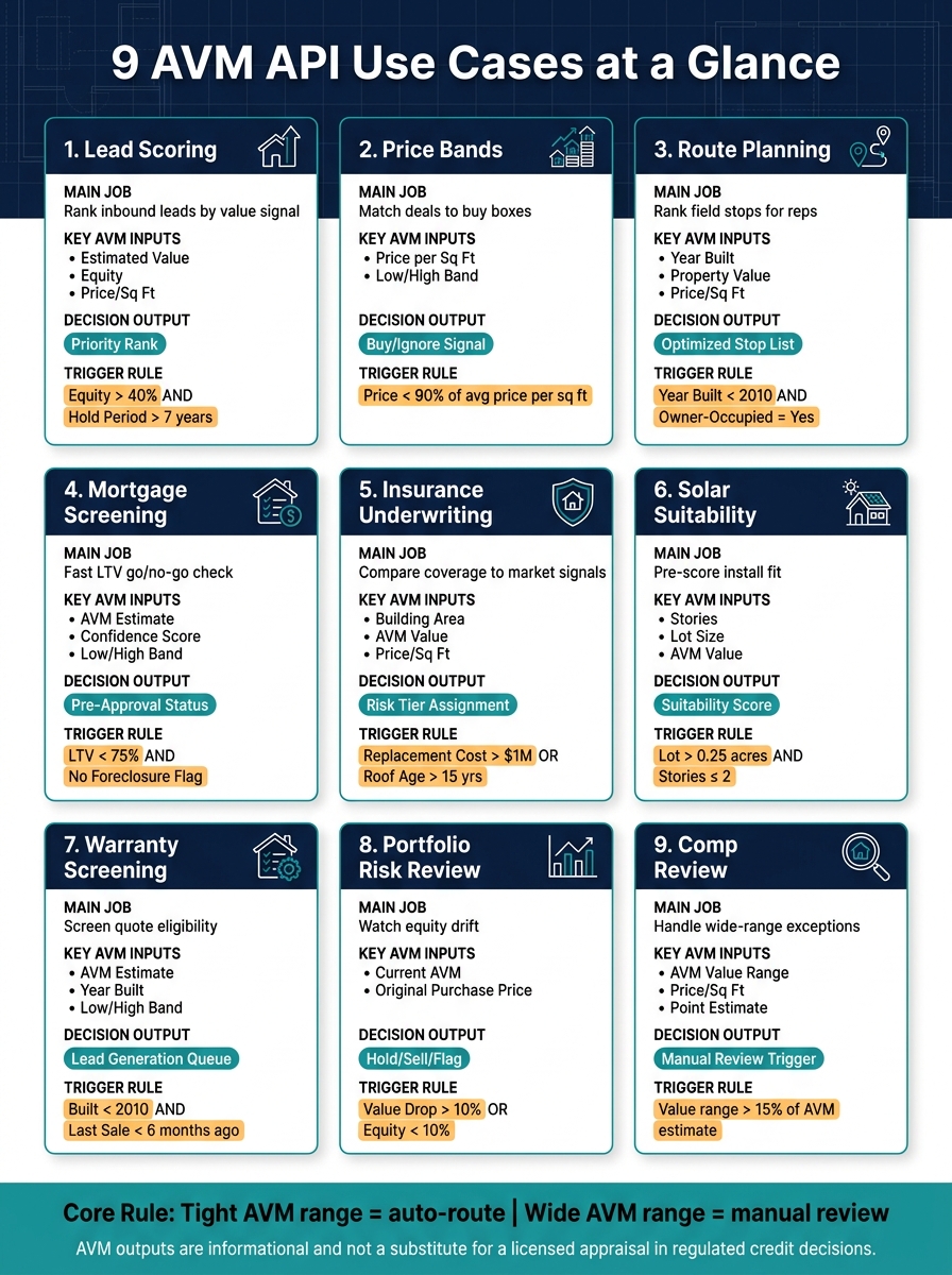
9 AVM API Use Cases: Inputs, Triggers & Decision Outputs
After the workflow breakdowns, these tables pull the nine AVM API patterns into one place. You can scan them to compare inputs, supporting fields, decision outputs, and trigger rules without jumping back and forth.
| Use Case | AVM Inputs | Supporting Data (BatchData) | Decision Output | Example Threshold |
|---|---|---|---|---|
| 1. Lead Scoring | Estimated Value, Equity | Ownership Type (LLC/Individual), Hold Period | Priority Rank | Equity > 40% AND Hold Period > 7 years |
| 2. Price Bands | Price per Sq Ft | Listing Status (Off-market/Active) | Buy/Ignore Signal | Price < 90% of average price per sq ft |
| 3. Route Planning | Year Built, Property Value | Owner-Occupied Status, Reachable Phone | Optimized Stop List | Year Built < 2010 AND Owner-Occupied = Yes |
| 4. Mortgage Screening | AVM Estimate, Confidence Score | Mortgage Balance, Last Sale Price | Pre-Approval Status | LTV < 75% AND No Foreclosure Flag |
| 5. Insurance Underwriting | Building Area, AVM Value | Construction Type, Year Built | Risk Tier Assignment | Replacement Cost > $1M OR Roof Age > 15 yrs |
| 6. Solar Suitability | Stories, Lot Size, AVM Value | Permit History, Property Type | Suitability Score | Lot > 0.25 acres AND Stories ≤ 2 |
| 7. Warranty Screening | AVM Estimate, Year Built | Contact Info (Phone/Email) | Lead Generation Queue | Built < 2010 AND Last Sale < 6 months ago |
| 8. Portfolio Risk | Current AVM, Original Purchase Price | Vacancy Status, Foreclosure Status | Hold/Sell/Flag | Value Drop > 10% OR Equity < 10% |
| 9. Comp Review | AVM Value Range, Comparable Distance | Sale Dates, Comparable Count | Manual Review Trigger | Value range > 15% of AVM estimate |
For implementation planning, the next table adds rough U.S. valuation context. This is where the numbers start to feel more concrete. Instead of just seeing a rule like LTV < 75%, you can picture how that rule plays out in lending, home services, insurance, and investor screening.
| Scenario | AVM Estimate | Requested Loan / Project | Calculated LTV / Margin | Value Range | Supporting Field |
|---|---|---|---|---|---|
| HELOC Screening | $525,000 | $100,000 (2nd lien) | 78% total LTV | +/- 4% | Mortgage Balance: $309,000 |
| Fix-and-Flip | $310,000 | $215,000 purchase | 31% gross margin | +/- 7% | Ownership Type: Individual |
| Roofing | $310,000 | $12,000 (roof) | 3.8% asset value | High | Reachable: Yes |
| Solar Install | $680,000 | $32,000 (10kW system) | 12-yr payback | High | Owner-Occupied: Yes |
| Portfolio Review | $1,250,000 | $900,000 balance | 72% LTV | +/- 3% | Foreclosure Status: None |
| Investor Scoring | $350,000 | N/A | 15% equity | $340k–$365k | Cash Buyer: True, Portfolio: 8 props |
| Home Warranty | $275,000 | $600 (annual plan) | N/A | $265k–$285k | Last Sale: 2024 |
| Insurance Review | $480,000 | $410,000 replacement cost | 85% coverage ratio | Medium | Construction Type: Wood Frame |
| Comp Exception | $405,000 | N/A | N/A | $380k–$420k | Nearest Comp: 0.4 mi |
A table like this helps in a very practical way. If you’re building an AVM-based flow, you don’t just need the property value. You also need the extra field that gives that value meaning in context, like mortgage balance for HELOC screening, owner-occupied status for solar, or foreclosure status for portfolio review.
Next, the conclusion ties these workflows into one AVM-centered stack.
Where BatchData Fits in an AVM-Centered Stack
The workflows above need a context layer around the AVM. Those nine use cases only work when AVM output is paired with ownership, contact, mortgage, and status data.
An AVM estimate tells you what a property is worth. It does not tell you who owns it, whether you can reach that owner, whether there are legal flags, or what data supports the estimate.
That’s where BatchData comes in. It adds the missing layer AVMs don’t provide: ownership, mortgage, listing, and status data.
For outbound sales and CRM scoring, Reverse Skip Trace connects a phone number or email to a person and property. It also adds DNC/TCPA flags, plus litigator and deceased indicators, which helps keep lists clean.
For valuation workflows, the Comparables API returns comp-level attributes and match controls. That makes AVM results easier to explain and bulk revaluations easier to run. In plain English, it turns a valuation estimate into something a team can actually use as a workflow trigger.
Conclusion
An AVM API is only as useful as what happens next. Across the nine workflows above, the same pattern shows up again and again: AVM outputs work best as triggers and filters, not as final answers.
The biggest gains come when you pair AVM output with property and owner data. Add ownership, mortgage, and contact data, and a simple value estimate becomes something far more useful: a routing decision.
Automate the clear-cut cases. Send edge cases to human review. And make sure every threshold is easy to explain.
FAQs
How accurate is an AVM API for real-world decisions?
AVM API output provides informational property data. It is not a professional appraisal. And because a licensed or certified appraiser does not prepare it, it can’t stand in for one.
For regulated uses like mortgage origination or credit decisions, you still own compliance and quality control. In practice, decisions are easier to support when the tool shows its logic and gives clear low and high value bounds, instead of relying on hidden model calculations.
When should a property go to manual review?
A property should move to manual review when a seller disputes an automated valuation or a partner wants to know how a specific number was calculated.
Manual oversight also matters for regulated activities like mortgage origination and credit decisions. In those cases, the valuation often needs to be explained in plain terms and backed up clearly for stakeholders.
What extra data should I combine with AVM results?
Combine AVM results with broader property and ownership data to get more context. BatchData can match AVM figures with ownership details, mortgage records, permit history, foreclosure status, and listing status, so you can see where a property sits in the market cycle.
For investing and outreach, adding investor profile data – like portfolio size, cash purchase history, and recent activity – helps you score leads with more precision and review risk with a clearer view.